Summary

Models are useful!

They summarize our data and allow us to explain it (build theories).

They allow us to predict what future data might look like.

Linear models are easy to fit.

If you can get away with a linear model, you should!

Non-linear models are really not that hard (except when they are).

An important difference is the time it takes to fit a linear model (fast, usually), relative to non-linear model (usually slow). This might become crucial, if you have a lot of data.

Non-linear models are almost arbitrarily flexible, but very flexible models might also be under-determined: this means that several different settings of the parameters set the model to be almost equally accurate. Leo Breiman calls this the “Rashomon effect”.

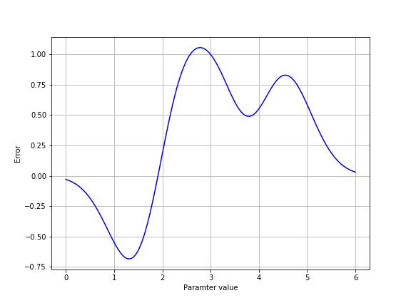
Another thing to beware are so-called local minima. These are settings of parameters that seem good, but only because all similar settings are worse. There might be completely different settings that lead to an even better global minimum.

One way to overcome local minima is by running the model fit several times with different initial conditions, finding the least error in all the different runs. This can be done by using the p0 key word argument when calling opt.curve_fit.

Default values

1. What is the default value of p0?
2. Is it different when you use opt.curve_fit with cumgauss and when you use it with weibull?
3. Write a function that performs “grid search” in the space of the parameters of the cumulative Gaussian function, sampling all parts of the space of possible parameters.

Check your model accuracy!

Cross-validation allows you to compare the accuracy of models that are very different from each other.

For further readings on this topic, please go to the reference section of this lesson.