Model evaulation with cross-validation

How do we know that a model is good enough?

In the previous section, we managed to reduce the SSE substantially relative to the linear model, by fitting a non-linear one, but it’s still not perfect. How about trying a more complicated model, with more parameters? Another function that is often used to fit psychometric data is the Weibull cumulative distribution function, named after the great Swedish mathematician and engineer Waloddi Weibull

def weibull(x, threshx, slope, lower_asymp, upper_asymp):
    """
    The Weibull cumulative distribution function

    Parameters
    ----------
    x : float or array
       The values of x over which to evaluate the cumulative Weibull function

    threshx : float
       The value of x at the deflection point of the function.
       For a lower_asymp set to 0.5, this is at approximately y=0.81

    slope : float
        The slope of the function at the deflection point.

    lower_asymp : float
        The lower asymptote of the function

    upper_asymp : float
        The upper asymptote of the function.
    """
    threshy = 1 - (lower_asymp * np.exp(-1))
    k = (-np.log((1 - threshy) / (lower_asymp))) ** (1 / slope)
    m = (lower_asymp + upper_asymp - 1) * np.exp(-(k * x / threshx) ** slope)
    return upper_asymp - m

As you can see, this function has several more parameters to account for features of the data that may interest us.

Let’s see what that might look like:

fig, ax = plt.subplots(1)
ax.plot(x, weibull(x, 0.5, 3.5, 0.5, 0.95), label='threshx=0.5, slope=3.5, lower_asymp=0.5, upper_asymp=0.95')
ax.plot(x, weibull(x, 0.5, 3.5, 1, 0.95),  label='threshx=0.5, slope=3.5, lower_asymp=1, upper_asymp=0.95')
ax.plot(x, weibull(x, 0.5, 3.5, 1, 0.85), label='threshx=0.5, slope=3.5, lower_asymp=1, upper_asymp=0.85')
ax.plot(x, weibull(x, 0.25, 3.5, 0.5, 0.95), label='threshx=0.25, slope=3.5, lower_asymp=0.5, upper_asymp=0.95')
ax.plot(x, weibull(x, 0.75, 3.5, 1, 0.85), label='threshx=0.75, slope=3.5, lower_asymp=1, upper_asymp=0.85')
ax.grid('on')
fig.set_size_inches([14, 8])
plt.legend(loc='lower right')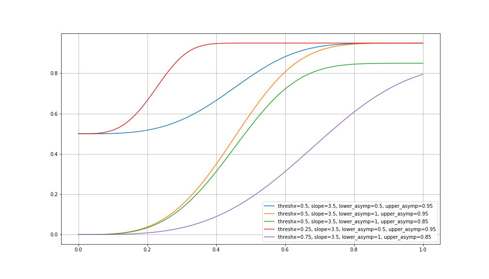

We go ahead and fit this function as well, using curve_fit

params_ortho, cov_ortho = opt.curve_fit(weibull, x_ortho, y_ortho)
params_para, cov_para = opt.curve_fit(weibull, x_para, y_para)

And examine the results:

y_ortho_hat = weibull(x, params_ortho[0], params_ortho[1], params_ortho[2], params_ortho[3])
fig, ax = plt.subplots(1)
ax.plot(x, y_ortho_hat)
ax.plot(x_ortho, y_ortho, 'bo')

y_para_hat = weibull(x, params_para[0], params_para[1], params_para[2], params_para[3])
ax.plot(x, y_para_hat)
ax.plot(x_para, y_para, 'go')

ax.grid("on")
fig.set_size_inches([8, 8])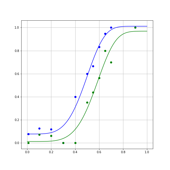

Calculating the error, we find that the SSE is smaller for this model:

SSE_para = np.sum((weibull(x_para, params_para[0], params_para[1], params_para[2], params_para[3]) - y_para) ** 2)
SSE_ortho = np.sum((weibull(x_ortho, params_ortho[0], params_ortho[1], params_ortho[2], params_ortho[3]) - y_ortho) ** 2)

Should we switch over to this model? It seems to be doing better in fitting the data.

Overfitting

One of the reasons we should be suspicious of the more accurate second model is that the Weibull function has more parameters. This is sometimes referred to as the “degrees of freedom” of the model, and intuitively just means that the more parameters a function has, the more adjustments you can make to the estimated \(y\) values that you could consistently get across a range of \(x\) values. Let’s examine the most extreme case of that. Consider the case of fitting a polynomial of degree 6 to these data (7 parameters, including \(\beta_0\)):

beta_ortho = np.polyfit(x_ortho, y_ortho, 6)
beta_para = np.polyfit(x_para, y_para, 6)

This model has even smaller error on the data:

SE_ortho = np.sum((y_ortho - np.polyval(beta_ortho, x_ortho))**2)
SSE_para = np.sum((y_para - np.polyval(beta_para, x_para))**2)

But examining the curves of the fits, you can see that it does some absurd things in order to fit the data:

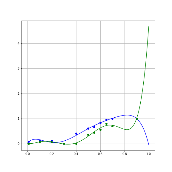
That is, it bends to match not only the large-scale trends in the data, but also the noise associated with each data point. This match to the noise that characterizes the sample is called “overfitting”.

Overfitting generally becomes worse as a model becomes more flexible. This can roughly be quantified by the number of parameters in the model. That is, a polynomial of degree 6 will always fit the data more accurately than a polynomial of degree 5, only because of overfitting to the noise in the sample.

Overcoming overfitting – model selection with cross-validation

One strategy to overcome overfitting is by separating the noise in the data used to fit the model from the noise in the data used to evaluate the model. This is called “cross-validation”. We fit the model to one sample, and then evaluate it on another. If we haven’t collected two separate samples, it might still be safe to assume that the noise in every individual observation (in the case of these experiments, each trial) is independent, and we can generate two samples by splitting the data up into sub-samples. There are different ways to split up the data, but in this case it makes sense to separately look at odd trials and at even trials, minimizing serial order effects (such as how tired the person got).

We refer to the sample used for fitting the model as the “training set”. Using the training set, we find the parameters of the model

ortho_1 = ortho[::2]
x_ortho_1, y_ortho_1, n_ortho_1 = transform_data(ortho_train)
params_ortho_1, cov_ortho_1 = opt.curve_fit(cumgauss, x_ortho_1, y_ortho_1)

The left-out sample is called the “testing set”. We use this sample to calculate the error:

ortho_2 = ortho[1::2]
x_ortho_2, y_ortho_2, n_ortho_2 = transform_data(ortho_train)
SSE_ortho_2 = np.sum((cumgauss(x_ortho_2, params_ortho_1[0], params_ortho_1[1]) - y_ortho_2) ** 2)

In order for this to be cross-validation, we would want to also do it the other way around: use set #2 as the training set and evaluate on the set #1 as the testing set:

params_ortho_2, cov_ortho_2 = opt.curve_fit(cumgauss, x_ortho_2, y_ortho_2)
SSE_ortho_1 = np.sum((cumgauss(x_ortho_1, params_ortho_2[0], params_ortho_2[1]) - y_ortho_1) ** 2)

To evaluate model over all

Next, let’s summarize the points we learned. We’ll also see a list of resources for further learning about the topics we discussed.

Click here for the next section.